Response geometry explains adversarial robustness

Defending against adversarial attacks is critical for modern AI applications. Here I describe how we can use response geometry to predict a neuron’s susceptibility to attacks.

This writeup builds on my previous post about using the curvature of a neuron’s response surface to understand its behavior. If that idea is unfamiliar to you, then I recommend reading that post before this one.

Adversarial examples

Adversarial examples are a worst-case demonstration of artificial neural networks’ (ANNs) inability to gracefully cope with shifts or distortions of their inputs. To construct one, an adversary must modify, or perturb, the input in a very small but specific way such that the output of the ANN changes significantly. The figure below is adapted from an iconic example provided in one of the first papers demonstrating adversarial attacks on ANNs, authored by Dr. Christian Szegedy and colleagues. The original input images are in the left column and they belong to the categories “mantis” and “dog.” The images in the middle column are adversarial perturbations that can be added to the original inputs to produce adversarial images in the right column. All of the adversarial images are labeled as “ostrich” by the network. The perturbations have to be magnified to allow you to see what they look like because their original scale is at the lower bound of what a typical computer image can convey.^† Importantly, these attacks do not just apply to images. They have been demonstrated to work pretty much anywhere that ANNs are useful, and they almost always seem innocuous or are imperceptible to a person. Successful demonstrations include tricking text analyzers that are used for product review summaries, social media feeds, and search result rankings; tricking smart home devices to execute a command; and tricking a self-driving car to mistake a stop sign for a yield sign.

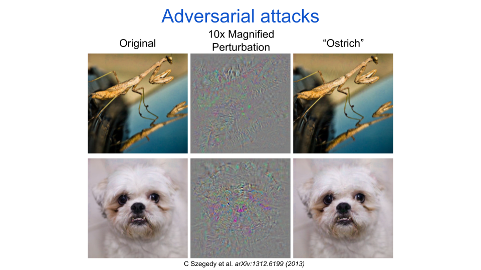
fig. 1 Natural images (left column) can be modified by small perturbations (middle column, magnified) to produce adversarial images (right column). The adversarial images are confidently misclassified by the neural network.

To be more precise, adversarial perturbations are modifications of the input of a network that are small in magnitude, but cause a big enough shift in its output to change its behavior. While it is not a hard requirement, they are also often semantically unrelated to the new output of the network – for example the “ostrich” perturbation is not recognizable as an ostrich. These two criteria, small size and uninterpretable semantic quality, are what makes them so interesting to researchers. There are adversarial perturbations that could trick a classifier in an uninteresting way, such as adding a horizontal stroke to a “0” to trick a classifier into calling it an “8”, or putting wheels on a canoe to trick the classifier into thinking it is a bicycle (or is it a bicycle disguised as a canoe?). If these obvious attacks were what was demonstrated by Dr. Szegedy and colleagues then few other researchers would have paid attention. Unfortunately, we do not have a good way to measure “semantic quality,” so the research community can only use the average size of the perturbations to quantify adversarial robustness, which indicates how much a network can handle adversarial attacks. However, they do often also show examples of perturbed inputs to allow readers to judge for themselves whether the semantic content is reasonable given the original and new network outputs. Now that we have defined the adversarial attacks and robustness we can better understand how such attacks are created.

Following gradients

There are many methods for constructing adversarial perturbations and they can roughly be categorized by how much access they have to the network they are attacking. All of the methods, however, seek the same goal: to maximally change a function’s output given a minimal change in its input. To illustrate how attackers achieve this, let’s consider an example where the function input is the position on a map and the function output is the elevation at that position. We can summarize such a function with a topographic map. Topographic maps use iso-elevation lines to indicate altitude, which means your elevation is constant if you walk along the line. This is illustrated in the following figure:

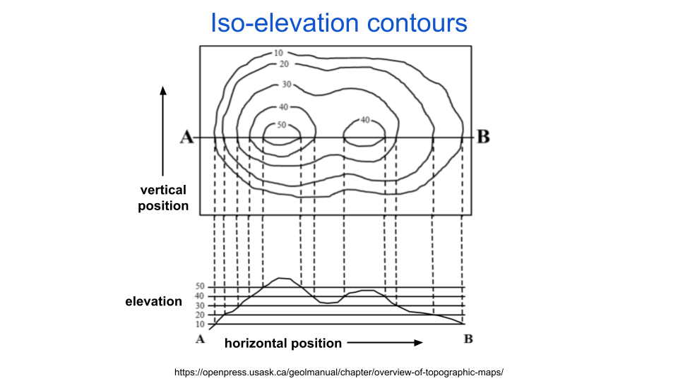
fig. 2 Topographic maps indicate altitude with iso-elevation lines.

Following the goal we defined earlier, we want to determine how to minimally change our position and maximally increase our elevation. There are two things to consider to solve this: one is where to start and the second is what direction to walk from there. In the case of adversarial examples the starting position is fixed to be the original input, like the dog or mantis above. In the figure below I indicated a starting position with a smiley face. The optimal direction to climb at any given position is orthogonal to the iso-elevation lines. This orthogonal direction aligns with the maximum gradient of the function, which is a term in math that has an intuitive mapping on to gradients in common language, such as a temperature gradient or the grade of a hill. That is to say that the gradient indicates how much the function’s output changes for a given minimal directional change in the function’s input.

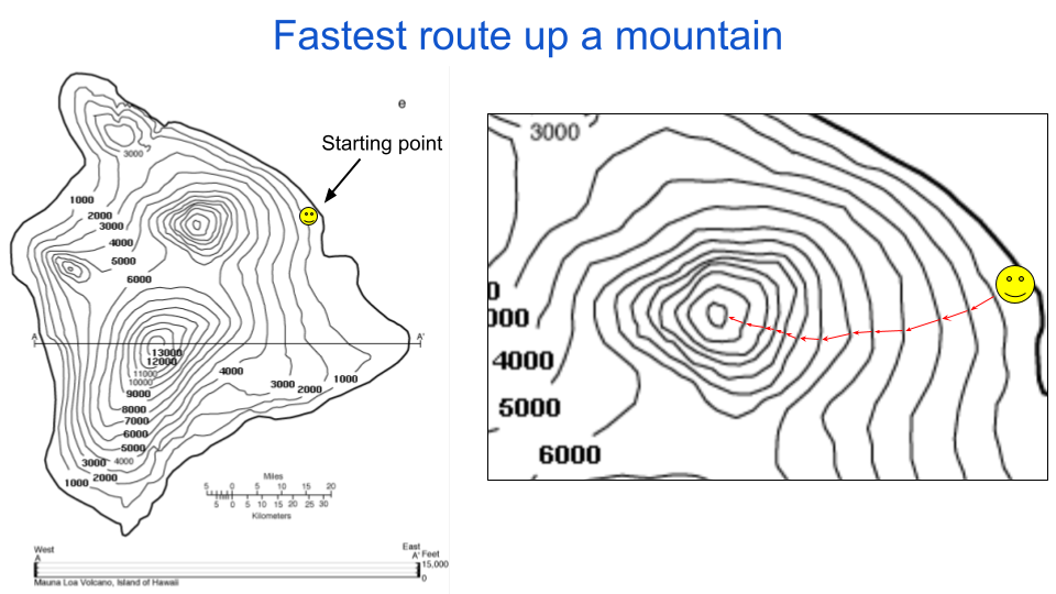
fig. 3 A path that is orthogonal to the iso-elevation lines on a topographic map is the fastest way to change altitude.

All methods for finding adversarial examples are derived from this same guiding principle, which is to use gradients (or approximations thereof) to determine what direction to go. I’ll explain in the wrap-up that this is considered a local perspective on finding an optimal path. In my previous post on iso-response contours, I explained how images can be thought of as arrows reaching to points in a high-dimensional space. Along this line of reasoning, an adversarial perturbation can be drawn as an arrow extending from the original input with some direction and magnitude. This is the same concept that we are using in figure 3: each red arrow starts at some position and ends at some other position. And just like each point on that map has an analogous location in the world (in this case Hawaii), the points in our neuron response figures have analogous images. To determine the input perturbation that maximally changes a function’s output, we choose arrow directions that are orthogonal to the function’s iso-response contours. Usually that function is an entire neural network, but the explanation also applies to single neurons.

Neuron robustness

Scientists use a large variety of different types of models to describe neurons in both neuroscience as well as artificial intelligence research. One way to organize the models is by their level of abstraction, which describes the tradeoff between biological accuracy and computational complexity. Indeed, one major goal of computational neuroscience is to discover the level of abstraction that has minimal complexity while still emulating the behavior of biological organisms. A neuron’s response surface geometry can help us quantify differences in behavior, such as a model’s selectivity, invariance, or robustness. It can also help us understand complexity, in that neurons with straight iso-response contours are minimally complex and so any deviation from straight contours will indicate more complex (or conversely, less linear) processing. The above climbing example maps well to how we will use iso-response contours to understand neuron robustness. Let’s consider two models: one that produces straight iso-response contours and one that produces outward (i.e. away from the origin) bent iso-response contours. The next figure shows the iso-response contours for these models as well as the arrows indicating optimal adversarial perturbation directions for increasing their response with minimal perturbation size.

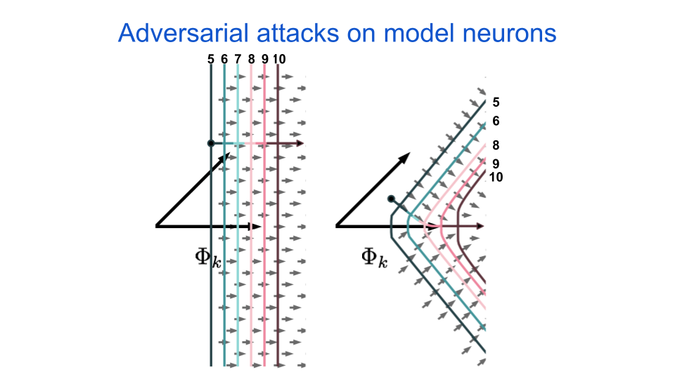
fig. 4 Two neurons are simulated and their iso-response contours are shown. The numbers above the response indicate the neuron’s activation in arbitrary units. The little gray arrows indicate the maximal gradient direction for increasing the neuron’s activation. The longer colored arrow indicates an optimal path taken from the point indicated by the black dot.

The longer colored arrows in the above figure indicate an optimal adversarial perturbation from a given starting point. The \(\Phi_{k}\) variable indicates the direction of the neuron’s maximally exciting image, or MEI. As the name implies, this image tells us what feature the neuron is most excited about in the world. In biological and artificial neural networks, the MEI features vary in complexity as one ascends a hierarchy of processing stages, from simple edges at the lowest levels to faces and complex objects at the highest levels. Both neuroscientists and artificial intelligence researchers often use a neuron’s MEI to label that neuron, for example as a “vertical edge detector” or a “dog detector.” All of this matters when we think about an adversarial attack on the neuron.

For both neurons, as we take steps in the adversarial direction, the output will look more and more like the neuron’s MEI. However, this will happen faster for the neuron with the curved response contours, to the point where the input eventually just ends up looking exactly like the MEI. This means that the optimal perturbation direction for neurons with curved response contours is more aligned with their MEIs than for neurons with straight contours. Thus, if we assume that neurons are interested in semantically relevant features, then we hypothesize that the resulting adversarial perturbations are going to be more semantically relevant if the neurons have curved response contours. And as I discussed earlier, if we modify a picture of the number “0” to look more like an “8,” then we should not be too surprised if a neuron that has an MEI that looks like an “8” gets more excited.

It turns out that the curved contours can result in larger overall perturbation magnitudes when we have a network of these neurons as well. This is because an ensemble of neurons with bent contours will constrain the adversary, thus limiting its perturbation options. The next figure demonstrates the idea, where we show all possible pixel values that will result in an increased activation for neuron \(k\).

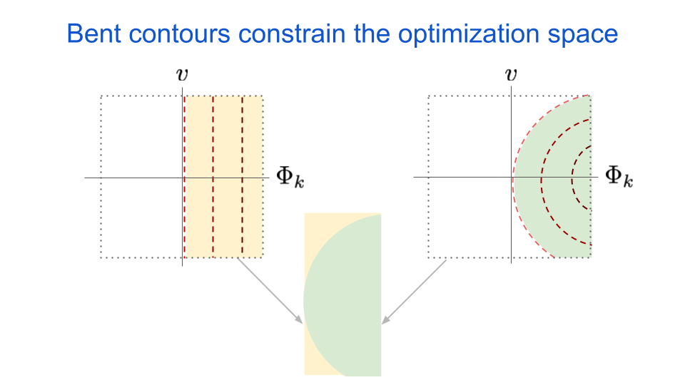
fig. 5 Inputs from the shaded region will have increased activation when compared to inputs not in the shaded region. By restricting the shaded region, bent iso-response contours constraint the space of possible inputs to increase a neuron’s activation.

The dotted box represents the range of allowable pixel values for input images. The yellow shaded area represents all possible inputs that would increase the activation of neuron \(k\) if it had straight iso-response contours, relative to the non-shaded area. Conversely, the green shaded area represents all possible inputs that would increase the activation of neuron \(k\) if it had bent iso-response contours. As you can see when we overlay the two shapes, any amount of bending will reduce the number of possible inputs that have an increased response. This means an adversary will have fewer options to choose from if it wishes to increase the output of neuron \(k\).

Wrap up

At a high level, adversarial examples are one of many pieces of evidence supporting the idea that ANNs don’t perceive the world like we do. Given that there are other mismatches, exclusively solving adversarial susceptibility in ANNs is unlikely to align human and machine perception. However, adversarial examples still serve as a valuable test of ideas in neural computation: if we have an idea to explain perception, then our model of the idea should be robust to adversarial attacks.

In this post I explained how we can use the iso-response surface of a neuron to determine adversarial robustness. This might be intuitive for you if you think about a counter-example: what should we do if we wanted to change an input to minimally change the output? The answer is to follow the iso-response contours. Therefore, moving perpendicular to the iso-response contours will have the opposite effect. Following this intuition, we hypothesized here that the outward bent contours will result in larger adversarial images that look more semantically meaningful. I go into more detail in my paper, where I present supporting experimental evidence using multi-layer neural networks.

One detail that would be remiss of me to ignore is the spacing between the iso-response contours. You might have noticed that the bent and straight contours in figure 4 were (approximately) equally spaced. The optimal adversarial perturbation direction at any given point is indeed orthogonal to these contours. However, if the spacing is not guaranteed to be equal then there may be a suboptimal direction to take at that moment that ultimately achieves the goal with fewer steps. If you wish to climb a mountain in as few steps as possible, for example, you might need to walk in a sub-optimal direction for a little while to get to a cliff face that will let you climb at the fastest rate. This distinction is subtle, but important when we are trying to build defenses against adversarial attacks. The difference I’m describing is between a local and a global optimization process. Importantly, though, a global perspective, such as knowing that there is a cliff on the other side of some valley, is rare when attacking neural networks because of the high dimensionality of the inputs.

Thus, iso-response contour curvature provides part of the story of adversarial susceptibility, and iso-response contour spacing provides another part. No one has provided a complete picture of adversarial vulnerability using iso-response geometry, and so we do not know if there are more aspects to consider. However, there has been some excellent progress recently. Hopefully this post increased your understanding and demonstrated yet another way that the geometry of a neuron’s response surface can teach us about how that neuron processes its inputs.

Footnotes

† Computer images are composed of pixels that each take on one of 256 possible values. This is the same as saying that they are 8-bit images. If one were to rescale the pixel values to be between 0 and 1, then the average pixel perturbation size for the examples from Szegedy et al. is 0.006. This corresponds to changing a single pixel by about 2, or in reality changing many pixels by less than 1. As such, adversarial perturbations are often smaller than the available bit-depth of current displays.