Understanding neurons using response geometry

Scientists have long summarized neurons in terms of the relationship between their inputs and outputs. Here I describe a technique that allows us to go beyond previous approaches to succinctly describe important and complex neural behavior.

Neuron selectivity and invariance

An important computational goal of the early visual pathway, from the retina to the primary visual cortex (V1), is to produce a representation of visual features that are useful for downstream tasks, like navigating the world and identifying objects. In order for a V1 neuron’s output to be decoded by downstream brain areas, it must reliably modulate its response with respect to certain variations in the visual world and remain constant for others. For example, let’s suppose we live in a binary edge world, where all scenes are made up of combinations of oriented edges. In such a world, images of vertical edges would occur when a column of 1s immediately precedes a column of 0s, or vice versa. To encode such a world, our brain might want to have a “vertical edge detector” neuron that signals the presence of any vertical edges. This means we want our neuron to be selective for the presence of a vertical edge, as opposed to other orientations, but invariant to the phase of the edge, i.e. whether it is 0s followed by 1s or the other way around. In neuroscience, such a neuron is called a complex cell and is a common basic cell type.

It was precisely the discovery of analogous neuron types in the visual cortex of cats that led scientists to hypothesize that the brain is wired up to perform computations on signals coming from the world. This discovery occured in the late 1950s and created a revolution in neuroscience research. About twenty years later a scientist named Dr. Kunihiko Fukushima proposed a computer model to emulate the discovered behavior. His invention, called the neocognitron, was one of the earliest ancestors of modern day deep neural networks. One of the defining elements of the neocognitron were “C-cells”, which were designed to be selective for features in the world, but invariant to their position. In modern artificial neural networks, we often label neurons by what they are most selective for, such as snout or car detectors, and we explicitly engineer components that create invariance, such as pooling. Today, scientists have a variety of methods to measure and quantify selectivity and invariance in both biological as well as artificial neurons. These measurements are extremely important for developing an understanding of how we process information, and are often used to categorize neurons into groups. This blog post aims to explain one such method, which is primarily used in neuroscience and relies on characterizing the geometry of a neuron’s response surface.

The neural response surface

First, an obvious statement: neurons receive signals as input and produce signals as output. Let’s assume that some target neuron receives input from 100 other neurons, and produces a single output that might be read by any number of downstream neurons. Going forward, we will define the target neuron as the neuron that we are currently interested in studying, and we will indicate it mathematically with the index \(k\). Let’s assume that the target neuron will produce an output for any combination of signals coming from the 100 input neurons. Or, put another way, the target neuron is a function that maps a 100-dimensional input to a scalar (i.e. a single number, which would then be single-dimensional) output. The neural response surface is a description of the neuron’s output for all possible combinations of inputs.

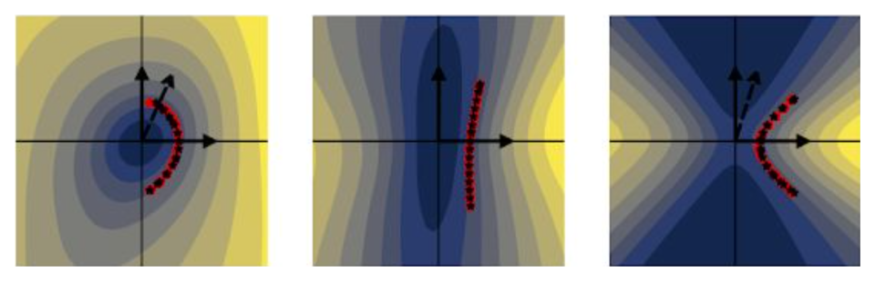
It is impossibly difficult to measure the entire response surface of a neuron, even in the case of modern artificial neural networks. However, if we assume that the response surface is relatively smooth and regular, then we can still learn a lot about the neuron by looking at cross sections, which are much more tractable to estimate. This presents our next challenge of choosing which cross sections to take. Just like cutting an onion in half, one type of cross section will reveal a different structure from another one.

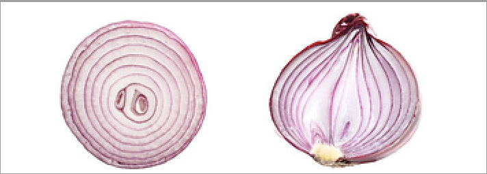
fig. 1 Taking cross sections of complicated surfaces can reveal structure, but the structure looks different depending on the orientation of the cross section.

Instead of input from other neurons, let’s consider a neuron that receives images as input and produces a scalar output. Individual input images can also be thought of as points in a high dimensional space. For example, a 10-by-10 image thumbnail has 10*10=100 pixels. Therefore, we can equivalently think of the image as a point in a 100-dimensional space. Each dimension can be represented as an axis, where the position along the axis is the value of the pixel. If individual pixels are allowed to be numbers between 0 and 1 (like in a grayscale image, where 0 is black, 0.5 is gray, and 1 is white), then all allowable images exist in a 100-dimensional cube. Just to really drive this idea home – every single point in the 100-dimensional cube is also an image. The next figure has an illustration of a 3D image space with such a 2D cross section drawn in light gray. If we draw arrows starting from a single origin such that the tips reach two image points, then we can compute the angle between the arrows to determine how similar those images are. If two image arrows are perpendicular, then they are maximally dissimilar from each other.

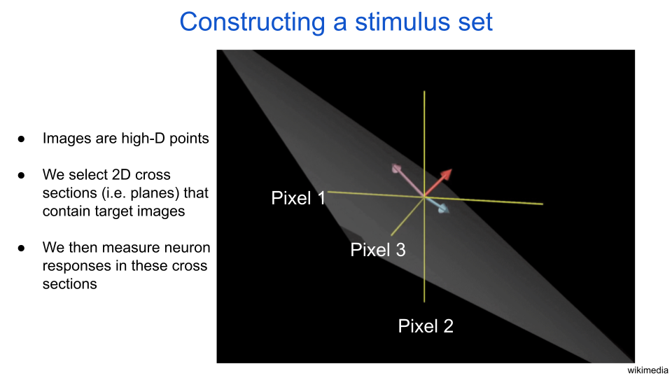
fig. 2 Images are high-dimensional points. In this illustration, each yellow axis represents the value of a pixel for a three-pixel image. The gray sheet represents a cross section, or plane. The purple and blue arrows define the cross section. The red arrow points in the remaining direction, which is perpendicular to the cross section.

Here’s a roadmap of what is to come: To explore the response geometry of our target neuron, we will first take a two-dimensional cross section of the high-dimensional input space. Next we will discretize the cross section, that is to say we will sample the cross section with a tiling of points evenly spaced from the minimum allowable pixel value to the maximum. Then we will measure the output of the neuron for each of the images selected from the discretization process. Finally, we will measure the curvature of the response surface to quantify selectivity and invariance of the neuron.

Choosing a cross section

We are interested in the behavior of the target neuron for images that it cares about, or ones it would see in its natural environment. As such, we shouldn’t use just any old cross section to analyze a neuron, but instead cross sections that contain images (i.e. points) that are relevant for that neuron. Cross sections are defined by two vectors, which are mathematical objects that point in a particular direction in space and are drawn as arrows. If we set at least one of the vectors to be pointing in the direction of an image that the neuron cares about, then we know that the cross section at least partially contains interesting inputs for the neuron. The next figure illustrates how each point in the grid can be reshaped to be visualized as an image. A few of the points around the edges are displayed as images. Notice how these images have some structure to them and are systematic in how they look. For any given cross section, all of the images are coplanar, which is to say that they can all be described as a linear combination of two exemplar images. This idea of linearity is also illustrated in the figure below in that all of the corner images can be constructed by adding two of the center images.

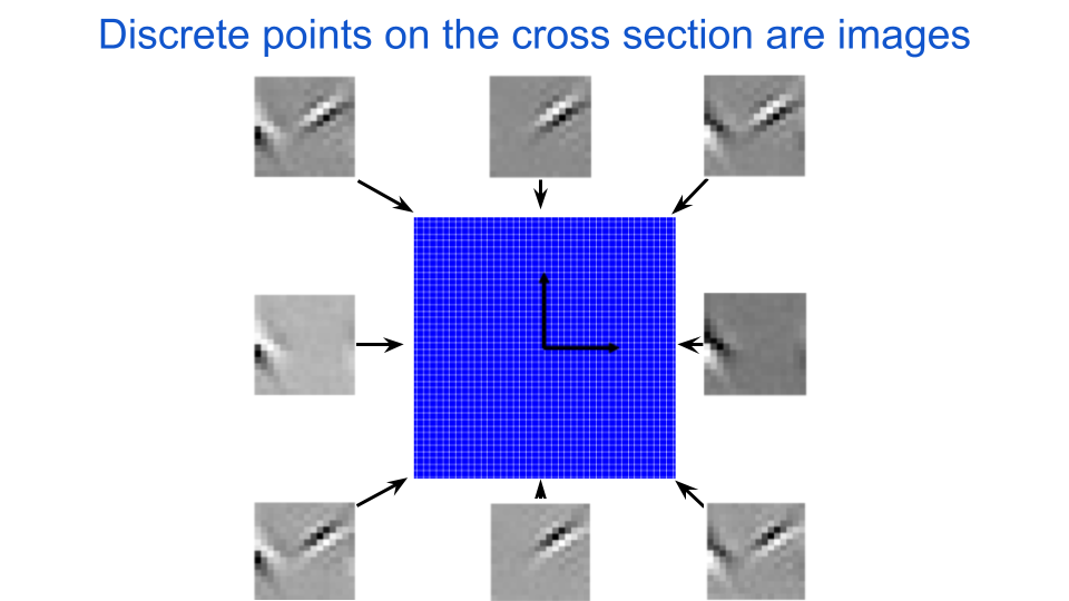
fig. 3 We discretize a cross section of the input space into a two-dimensional grid and collect the points to define a dataset of images. The black arrows are perpendicular vectors that define the cross section. The origin for all of the cross sections we consider here will be a zero-contrast image, in other words a uniform gray image.

In addition to constraining our input space to be coplanar, we are also going to constrain our output space to simplify the analysis. Specifically, we are going to look at the curvature of the iso-response contours of the neuron. These contours are connected points that all produce the same (hense “iso”) output from the neuron and they all exist on the cross section. To see the iso-response contours, we will compute the neuron’s activity (i.e. its output) for all of the cross section images and then recolor the points according to the activity.

As I said before, we want to pick a cross section that is relevant for our neuron. To do this we define one of the two cross section axes as the neuron’s maximally exciting image (MEI), which is an image that was optimized to look like the feature in the world that is most interesting to the neuron. There are a lot of ways to find a neuron’s MEI in neuroscience and in artificial neural network research, but for now let’s leave aside how the image was produced and just assume it is representative of what the neuron likes most. Going forward, we will represent the MEI with the symbol \(\Phi_{k}\), where the \(k\) tells us it is the MEI for the \(k\)th neuron in our assembly. For now the other axis can be any random orthogonal (i.e. perpendicular) image, but we will choose more specific orthogonal images later.

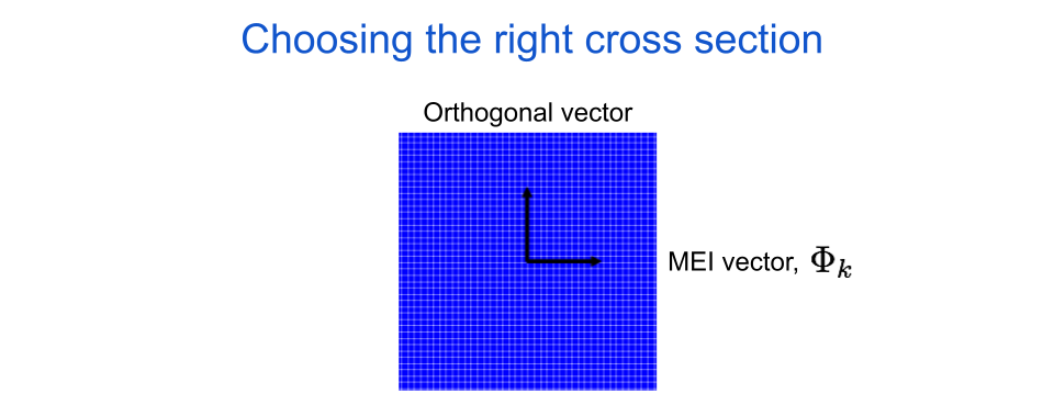
fig. 4 The horizontal axis for an image cross section is always the target neuron’s maximally exciting image, or MEI.

Plotting the contours

We can now color the points according to the neuron’s activity, \(a_{k}\). Visualizing the iso-response contours is easy, we just collect the output values into a fixed number of bins and then the bin boundaries will lie along iso-response contours. Here’s what it would look like for a simple linear neuron:

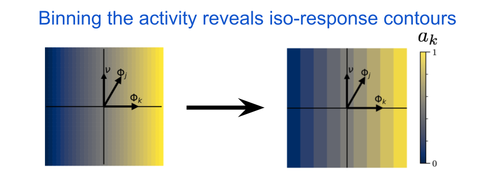
fig. 5 The iso-response contours for a linear neuron are straight and orthogonal to the neuron’s MEI, \(\Phi_{k}\). In this image, \(\Phi_{j}\) indicates the MEI for some other neuron and \(\nu\) indicates the chosen orthogonal axis. For a linear neuron, the iso-response contours will be straight regardless of the chosen direction for \(\nu\). The color indicates the output activity of neuron \(k\), where blue is low and yellow is high.

Notice how the lines are straight and orthogonal to \(\Phi_{k}\). This will be true for any linear system, and it means that the neuron is insensitive to orthogonal perturbations away from it’s preferred input. What happens if we apply a pointwise nonlinearity to our neuron’s output? A pointwise nonlinearity is a function that maps a single scalar to another scalar, and therefore a pointwise nonlinear neuron does not interact directly with its neighbors in a given layer. This is exactly the type of operation that is used in almost all standard deep neural networks: a linear operation followed by a pointwise nonlinearity. For example, in the next figure we include the Rectified Linear Unit (ReLU) nonlinearity, which sets all values below some threshold to zero and then acts as an identity mapping (i.e. output equals input) for all values above that same threshold.

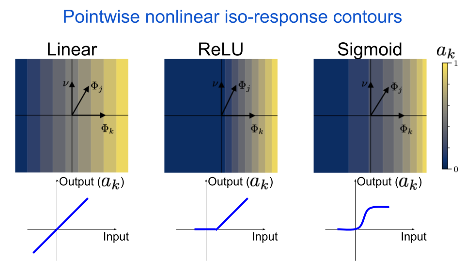
fig. 6 The iso-response contours for a pointwise nonlinear neuron are still straight & orthogonal to the neuron’s MEI. The nonlinearity can only change the spacing of the lines, or set values to zero.

We can see that the iso-response contours are still straight. This is because the nonlinearity is applied after the linear operation, and so the nonlinearity can only change the spacing between the lines. This is true for all types of pointwise nonlinearities, which we demonstrate by also including a sigmoid nonlinearity.

Straight vs. curved contours

Biological neurons tend to have more complicated iso-response contours, as well as some more sophisticated artificial neural network neurons. Specifically, the contours tend to have curvature in the sense that they bend towards or away from the origin. Since linear neurons produce straight contours, it is reasonable to think about curvature as indicating a deviation from linearity – more curvy contours indicate less linear functions. Additionally, let’s differentiate between outward curvature, which means it’s bending away from the origin, and inward curvature, which means it is bending towards the origin. One reason curvature is significant is because it tells us about what variations in the world the neuron is selective for and invariant against. To understand that better, let’s consider a few different types of coplanar perturbations that we can make from an input image. Here is a list of some options for a starting image along the horizontal axis:

• Right, toward the neuron’s MEI, then the target neuron’s activity will grow
• Left, away from the neuron’s MEI, then the target neuron’s activity will shrink
• Up, orthogonal to the neuron’s MEI, then the target neuron’s activity will change differently for each curvature type
• Along the iso-response contour, then the target neuron’s activity will not change

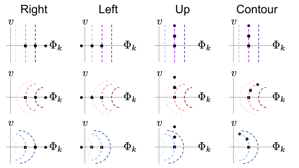
fig. 7 Visualizations of four out of many possible perturbation directions. For each direction, assume we start with the image depicted by the square, then perturb to the pentagon, then again to the circle. Straight contours are indicated in shades of purple, outward bending in shades of red, and inward bending in shades of blue. Darker colors indicate higher neural activation.

For linear neuron & pointwise nonlinear neurons, the last two directions are equal. But they are not equal for neurons with bent iso-response contours. What does this tell us? Each of the perturbation options above can be thought of as an experimental condition. We will look at the results from two such experiments to visualize the difference between straight and curved contours.

Experiment 1: Noise perturbations

To start we will look at the “up” perturbation condition for straight and outward bending contours.

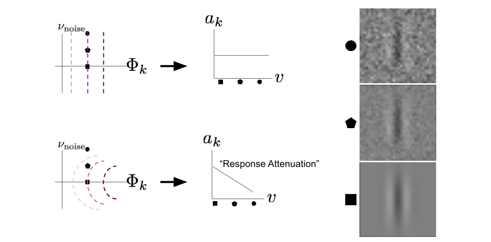
fig. 8 The “up” perturbation direction reveals an important difference between neurons with straight contours and neurons with outward curved contours. The orthogonal, \(\nu_{\text{noise}}\) axis is chosen to be a noisy image. The line plots in the middle indicate the response of the neuron (vertical axis) for each image type (horizontal axis). Each perturbation point is displayed on the right.

To start, we have two neurons with identical MEIs, but different curvatures. The vertical axis that helps define our cross section, \(\nu_{\text{noise}}\), is a random noise image. This means that an “up” perturbation will result in the MEI looking more and more noisy. Again let’s consider the pointwise nonlinear neuron. What happens to the output if we take a fixed point on the \(\Phi_{k}\) axis and then perturb orthogonally in the up direction? Nothing; as expected, the response is flat. However, the neuron with outward curvature decreases its output, \(a_{k}\), as we perturb “up” in the \(\nu_{\text{noise}}\) direction. We call this response attenuation. This means the neuron is selective against orthogonal perturbations away from its preferred stimulus. In other words, outward bending contours reveal that the target neuron’s output contains more information about how close the stimulus is to its MEI than straight contours.

This is important if we consider what the “MEI” means. In both studies of artificial neural networks and biology, scientists use MEIs or something similar to label neurons and group them together. For example, if the MEI is a vertical edge, then we would label the neuron a “vertical edge detector”. As we perturb an image away from the MEI axis, it will look less like the MEI and more like the image \(\nu_{\text{noise}}\). For linear and pointwise nonlinear neurons, we can perturb images along any direction that is orthogonal to the neuron’s preferred stimulus as far as we want and the response will not change. However, for neurons with outward facing iso-response contour curvature, orthogonal perturbations will result in response attenuation. Therefore, the neuron outputs have a higher degree of correspondence to their preferred stimulus label, and thus their output carries more relevant information about the input. Another way to say all of this is to say that the outward curvature indicates increased selectivity, where the amount of selectivity is proportional to the amount of curvature.

Experiment 2: Phase perturbations

As another example of the utility of this analysis, let’s look at perturbations that are along the iso-response contour. Again both neurons will have the same MEI, but different curvature. In this case, let’s compare the neuron with flat iso-response contours to the one with inward curved iso-response contours. This time we will define the vertical axis to be a phase shifted version of the neurons’ MEI. There are lines that are defined by the transition between light and dark lobes in the image. If we shift the phase of the edge, then each line will continuously move to the left or right, depending on what direction we shift the phase. This is a continuous and non-linear process.

If we look at the images that lie along evenly spaced intervals of the contours we can see a clear difference between the two neuron types. The perturbations for the top neuron have similar behavior as in the first experiment. With increasing perturbations, the image will look less like \(\Phi_{k}\) and more like \(\nu_{\text{phase}}\). However, this transition is linear, which means you will see both phases superimposed on top of each other. It is not actually shifting the phase of the edge. The perturbations for the bottom neuron, on the other hand, result in a continuous phase shift. By definition, since these images lie along the iso-response contour, the output of the neuron is equal for all of them. This means that the bottom cell has phase invariance, while the top cell does not.

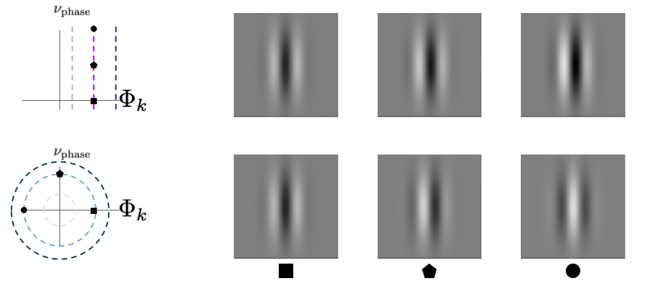
fig. 9 The “contour” perturbation direction reveals invariance for neurons with inward-bending iso-response contours. Perturbing along the top neuron’s iso-response contour will make the image look less like a linear combination of \(\Phi_{k}\) and \(\nu_{\text{phase}}\) instead of a phase shift. However, perturbing along the bottom neuron’s contour results in a phase shift. This is easier to see the farther along the contour we perturb, so we used larger perturbations here than those shown in figure 7.

Wrap up

These two experiments illustrate that iso-response curvature can indicate important information about how a neuron processes its input. The curvature analysis gives us a succinct way to understand the nonlinear function a neuron is performing, and allows us to know what features, or changes in features, that a neuron does and does not care about.

In summary, the big takeaways are:

• linear and pointwise nonlinear neurons have flat iso-response contours, regardless of the nonlinearity used
• flat iso-response contours indicate linearity and that the neuron’s response will not change if inputs are perturbed orthogonally from their preferred stimulus
• outward-curved contours indicate selectivity, and the amount of curvature will tell us how selective the neuron is
• inward-curved contours indicate invariance, which is a property of biological complex cells

There is much more that we can learn by looking at the curvature of neuron iso-response surfaces. In my next post, I use them to explain a concept in machine learning called adversarial robustness. If you are interested in digging into more details, check out my paper on the subject, as well as the work of James Golden et al. (PDF).